
Blog de diseño óptico
Telephoto
Telephoto
Ocular 10x Apocromático.
Mobile Phone Camera. 1G4P
In this link we can see another different design of the camera of a mobile phone. The fundamental differences are that in this one I use one less lens, 5 in total, being one of them of crystal and not of plastic. That means that this lens is totally spherical. I write the article again so that the reader has all the information on this page.
In the following article we will see how to perform the necessary calculations to design a mobile phone camera and I shall expose my own design of its own.
Designing a mobile phone camera phone is not a simple task.. In this case, we are going to design a system with an f/2.8 number with a 76º field of view.
The first thing to do is to choose the sensor we are going to use. In this case, I have chosen the OV16B10 sensor. It is a 16 megapixel sensor that can record in 4K at 60fps and zHDR at 30fps. In Figure 1 we can see the specifications of the product.

Figure 1. Sensor Specifications.
Once selected the sensor, we see that the pixel size is 1.12 microns, so the side color can not be greater than 1.12 microns. By looking at the image area, we can calculate the size of the image, since half the diagonal of the image area will be the height of the image.
Once we know the height of the image and knowing that the HFVO is 38º (half of the 76º of FOV), we can calculate the focal by means of a simple trigonometric rule. Figure 1 shows that the chief ray in the largest field cannot exceed 34.5º. This is very important to bear in mind when designing.
The MFT criterion is related to the Nysquit frequency of the sensor. In this case, the inverse of twice the pixel size will tell us the cutoff frequency. Also, we are going to calculate the size of the Airy disk, because it will tell us what should be the maximum size of the Spot Size RMS.
The minimum relative illumination is calculated through the rule of the cosine to the fourth, since it is related to the angle of incidence (which we know because it is the HFVO). Table 1 in Figure 2 lists all results.

Figure 2. Basic calculations.
Once we are clear about the objectives we have to achieve, we select the configuration of crystals we are going to use. In this case, we are going to use 1G4P, 1 crystal and 4 plastic lenses. These plastic lenses allow us extreme aspherical shapes. In Figure 3 we have the system report.


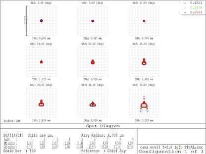

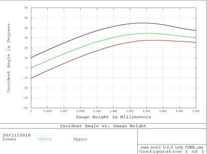

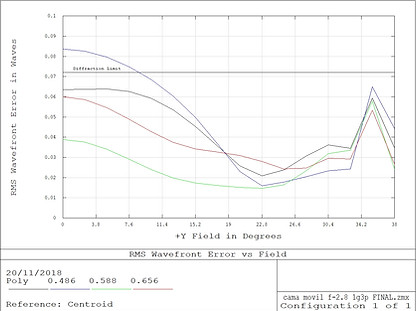


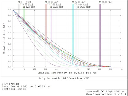
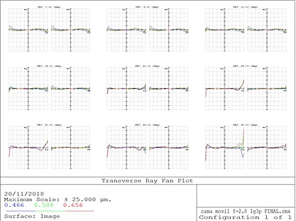


Figure 3. System report
The system consists of five lenses, the second being glass and the rest plastic lenses. The lenses used for this design are (in order); F52R-FDS18-F52R-F52R-F52R-F52R-N_SK11. This last lens is the parallel flat plate that serves not only as a protector for the sensor, but also acts as an infrared filter.
The system finally has a focal length of 4.20 mm, is very compact, barely measures 5.01 mm in length, a f/2.8 number and the size of the final image is 3.28 mm.
As can be seen from the diagram of Seidel's aberrations, the predominant aberration has been distortion. However, as a curiosity, during the design process the aberration that cost me the most to balance was the lateral color. Finally, the system has well compensated for all the aberrations and below the limits mentioned above. Let's review the system carefully.
In the FFT MTF graph we can see that at the spatial frequency of 223 cycles per millimeter the OTF module value corresponding to the diffraction limit is 0.564 (for both the tangential and sagittal plane values), this being the maximum figure that a perfect system would reach. The system presented reaches in axis an OTF module value of 0.46 (for both the sagittal and tangential planes). At mid-field, 20º the OTF module value is 0.45 for the tangential plane and 0.50 for the sagittal plane. At 38º degrees the OTF module value is 0.15 for the tangential plane and 0.42 for the sagittal plane. The system shows a really good performance, being the tangential planes of the fields of 38º and 34º happen to show the poorest outcome. The performance of the system can also be seen in the PSF graph.
We can continue checking the quality of the system observing that the distortion is well below 0.5% (when we had as top 1%) and the field curvature is less than 0.05 mm. At the bottom is the grid test graph to check for low system distortion.
The size of the Spot Size RMS is less than 4.4 microns in all fields except the 34º field, where it is 0.1 micron larger (in fact this is negligible) and the 38º field, where the point size is 2 times larger than desired. Even so, a very good image quality is to be expected in the whole field.
In the lower part of the report we can check the graphics of the Tranverse Ray Fan and the OPD. In the first one we see that the scale is 25 waves. I have used this scale because it is seen perfectly how all the fields are well compensated, but if we look at the edges of the graphs we see that they go up or down a little, because the system from 25º shows to be slightly affected by the comma aberration. This can be seen seeing the shape of the points in the graph of the spot size RMS. However, it is very small and the dot size is within the limits. The OPD graph has a scale of 0.5 waves, which indicates that the system is well optimized and has a good performance. In the graph of the RMS wavefront you can check again the quality of the system, with the polychromatism line below the diffraction limit line.
We had certain conditions to meet regarding side color value, relative illumination, and distortion. In the lateral color graph, the scale is restricted to 1.12 microns, which is the maximum value we could achieve, since the lateral color cannot exceed the pixel size. In this case it is much smaller, its maximum value being around 0.55 microns. The scale of the longitudinal aberration is very small and the three wavelengths pass at least twice through zero.
Another condition we had to meet was that the chief ray should not exceed 34.5º (if we exceed this value, the sensor manufacturer warns us that we are going to have vignetting and blurring in the images). In the graph "Incident Angle vs. Image Height" we can see that we did not exceed 34.5º, staying at 34º in the middle field, where we located the maximum value.
As far as the relative illumination is concerned, we can see that it is decaying until it reaches the minimum permitted value of 38%. In the simulation of the image we see that, in fact, the illumination decreases as we advance to the periphery. This lack of luminosity in the edge will be corrected later by the electronic circuit of the gain control.
In the graph "Diffraction Encircled Energy" and the PSF we see that almost all the irradiance falls on the first ring, as it should be, given that this is a system limited by diffraction.
If you found this article interesting, let me know. Below you can find my contact data.
Thank you very much! See you around!